이번 포스팅에서는 CVPR 2022에서 발표된 Jiayu Xiao et al.의 "Few Shot Generative Model Adaption via Relaxed Spatial Structural Alignment"를 읽고 정리해 보도록 하겠습니다.
1. Introduction
본 논문에서는 few-shot image generation을 다루고 있습니다. Few-shot image generation을 다룬 최근의 논문인 Ojha et al. 의 논문(IDC)에서 크게 두 가지의 문제점을 지적합니다. 첫번째는 identity degradation으로 source domain에서에 비해 target domain으로 전이되었을 때 identity가 떨어진다는 점입니다. 두번째는 unnatural distortion으로 현재 target domain에 잘 적응하지 못했을 때 발생합니다. 이는 IDC가 각각의 이미지의 고유한 구조를 보장하지 못해 target domain space의 sample들에 대해 drift 가 발생하기 때문입니다.
그래서 본 논문에서는 위 두 문제점을 해결하기 위해 relaxed spatial structural alignment (RSSA)를 제안합니다. RSSA는 identity degradation을 완화시키기 위해 source domain의 image로부터 구성된 보다 풍부한 spatial structure를 활용합니다. 그를 위해 두 가지의 cross-domain spatial structural consistency loss를 제안하는데, 하나는 self-correlation consistency loss와 disturbance correlation consistency loss입니다. Self-correlation consistency loss는 source 와 target generator의 feature map의 align을 돕습니다. 그로 인해 두 도메인간의 inherent structural information을 유지하려고 합니다. 한편, disturbance correlation consistency loss는 latent space 상에서 샘플들 간의 spatial mutual correlation을 align합니다. 그 결과 특정 샘플에서 variation tendency를 유지할 수 있게 됩니다. 위 두가지 loss term을 통해 target generator에서 생성된 샘플은 source domain에서의 self-correlation과 disturbance correlation을 유지할 수 있게 됩니다. 그러나, 이러한 alignment를 바로 적용하면 모델의 수렴이 늦어지게 됩니다. 그래서 본 논문에서는 latent space를 target domain에 가까운 subspace에 압축 시킵니다.
마지막으로, FID나 IS와 같은 전통적인 evaluation metric을 사용하는 대신 본 논문에서는 structural consistency score (SCS) 라는 새로운 metric을 제안하여 few-shot adaption 과정에서 identy preservation을 측정했습니다.
2. Method
2.1. Overview and framework
대규모의 source domain \(\mathcal{D}_s\)에서 학습 된 generator \(G_s\)가 있습니다. Generator는 target domain \(\mathcal{D}_t\)에 대해서 아래 수식으로 fine-tuning을 시킵니다.
\[L_G=-\mathbb{E}_{z{\sim}p(z)}[\log{(D(G_t(z)))}]\]
\[L_D=\mathbb{E}_{x{\sim}\mathcal{D}_t}[\log(1-D(x))]+\mathbb{E}_{z{\sim}p(z)}[\log{(D(G_t(z)))}]\]
적은 수(10)의 target domain으로 이루어진 few-shot setting 에서는 대부분의 fine-tuning이 오버피팅을 야기하기 쉽습니다. 그래서 본 논문에서는 다음 두 가지의 전략을 취합니다. 하나는 source domain의 이미지에서 유용한 structure prior를 보존시켜 adaption 도중에 identity degradation을 피하고, 다른 하나는 strucutral constraint를 완화하기 위해 source와 target domain에서 생성된 샘플들이 서로 가까워지게 하는 subspace에 latent space를 압축시킵니다. 아래 그림은 본 논문의 framework를 나타낸 모습입니다.

2.2. Cross-domain spatial structural consistency loss
이전의 연구(IDC)는 source와 target domain의 instance들 간의 상대적 distance를 유지하는 방향으로 sota를 달성했었습니다. 그러나 이 방법은 생성된 이미지들에서 왜곡이 발생하여 identity degradation이 발생했습니다. 그 이유로는 이전 연구에서 소개된 loss가 각 이미지의 고유한 구조를 보장하지 못하여 target domain space에서의 drift를 유발하기 때문입니다.

위 그림에서 IDC loss를 통해 빨간 점으로부터 파란점으로 adaption하여 상대적인 distance는 유지하였지만, 기존의 빨간 점으로부터 많이 벗어난 것을 확인할 수 있습니다. 위와 같은 상황에서 inherent spatial structure와 variation tendency를 유지하기 위해 본 논문에서는 cross-domain spatial structural consistency loss를 제안합니다.
2.2.1. Self-correlation consistency loss
본 논문에서는 몇몇 relevancy mining method에 영감을 받아 각 conv. layer에서의 feature map의 correlation matrix를 계산하여 이것을 image의 inherent structure information라고 formulate 했습니다. Source generator와 target generator의 같은 위치에서의 self-correlation matrix 쌍은 smooth-l1 loss로 규제되는데, 여기서 smooth-l1 loss는 Fast R-CNN에서 소개된 것으로 아래와 같은 형태를 띠고 있습니다.
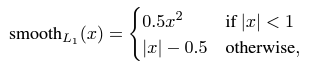
다시 돌아와서, smooth-l1 loss를 이용하여 source와 target self-correlation matrix의 차이를 좁혀 결국에는 비슷한 inherent structure를 갖도록 합니다.

2.2.2. Disturbance correleation consistency loss
Generative model의 latent space는 연속적입니다. 본 논문에서는 이미지들의 특정 disturbance에서 variation tendency를 알아보고자 하였습니다. 그래서 input noise vector를 anchor point로 잡고, 그 근방에서 batch를 뽑아내었습니다. 이러한 샘플들의 spatial similarities는 계산되어 source domain에서 target domain으로 transfer됩니다.
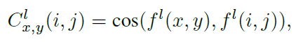
Input noise \(z_i\)에 대해 반지름 \(r\) 만큼의 이웃 영역을 정의할 수 있습니다 - \(U(z_i,r)=\{z{\vert}{\vert}z-z_i{\vert}<r\}\). 여기서 N개의 noise vector를 샘플링 하여 총 N+1개의 벡터로 이루어진 하나의 배치를 구성 할 수 있습니다. \(\{z_n\}^{N+1}_1\). \(D^l_{jk}\)를 배치에서 \(z_j, z_k\)를 입력으로 주었을 때 generator의 \(l\)번째 feature map 사이의 pixel-wise spatial mutual correlation이라고 정의하면, \(D^l_{jk}(x,y)\)는 feature vector상의 \((x,y)\)와 그에 따른 작은 region \(Q=\{(m,n){\vert}x-\delta/2<m<x+\delta/2,y-\delta/2<n<y+\delta/2\}\)에서의 similarity에 softmax를 취한 것과 같습니다.
수식으로는 아래와 같이 표현됩니다.


Disturbance correlation consistency loss는 이렇게 구해진 source와 target에서의 \(D^l_{jk}\)에 L1 loss를 걸어주는 방식으로 규제를 진행합니다. 따라서 spatial structural consistency loss \(L_{G_s{\leftrightarrow}G_t}\)는 다음과 같이 계산됩니다.
\[L_{G_s{\leftrightarrow}G_t}={\alpha}L_{scc}+{\beta}L_{dcc}\]
2.3. Latent space compression
앞서 소개된 spatial structural consistency loss는 source와 target domain에서의 alignment를 도와줍니다. 그러나 이런 loss를 바로 적용하는 모델의 adaption을 매우 느리게 만들어, 본 논문에서는 추가적으로 latent space compression을 제안합니다. 우선 Image2StyleGAN을 이용하여 target domain의 few samples \(\{x^t_i\}^n_{i=1}\)을 \(G_s\)의 \(W^+\) space로 invert합니다. 그렇게 되면 \(l\)번째 layer의 inverted latent code는 \(\{w^l_i\}^n_{i=1}\)로 표현이 됩니다. 이것으로 이루어진 n 열 행렬 \(A^l\)을 정의할 수가 있고, \(l\)번째 subspace \(\mathcal{X}^l\)를 구할 수 있습니다.
Input noise \(z_j\)가 주어졌을 때, 이에 상응하는 \(l\)번째 layer의 latent code는 \(w^l_j\)이고 modulation coefficient는 \(\alpha^l\)입니다. 본 논문에서는 이 \(w^l_j\)를 modulate하고 least square method로 \(l\)번째 subplane \(\mathcal{X}^l\)로 project합니다.

여기서 \(\hat{w^l_j}\)는 \(z_j\)를 projection한 것입니다. 위 방법을 통하여 원래의 latent space를 target domain에가까운 좁은 subspace에 압축합니다. 압축된 subspace에서 샘플링 된 latent code을 source generator에 입력으로 주면 생성된 이미지는 target domain의 몇몇 특징을 내포하고 있게됩니다.

사진에서 윗 줄은 original latent space에서 생성된 sample이고, 아랫줄은 FFHQ-> Sketches에서 압축된 subspace에서 생성된 sample입니다. 보다 Sketches 스러운 texture나 color를 갖고 있는 것을 알 수 있습니다. Alignment를 진행하기에 앞서 latent code를 sampling하는 것이 전체 학습 과정을 보다 빠르고 안정적으로 진행할 수 있게 됩니다. StyleGAN에서 convolution layer들은 서로 다른 semantic level을 담당하기 때문에 본 논문에서는 top-level에는 큰 \(\alpha_i\)를, bottom-level에는 작은 \(\alpha_i\)를 주어서 원본의 spatial structure는 최대한 유지하면서 high-semantic level의 attribute를 변경하고자 하였습니다.
2.4. Evaluation metric
전통적으로 FID와 IS는 GAN을 평가하기에 많이 사용되어 왔습니다. 그러나 둘다 Inception network를 거치는 데, 이는 spatial structure를 측정하는데는 적합하지 않습니다. 게다가, few-shot setting이기 때문에 학습 이미지와 유사한 이미지를 생성해내는 경우가 많은데 이런 경우 IS가 높게 나와 직관과 반대되는 경향이 나타납니다. 또한, FID는 많은 수의 실제 이미지를 요구하는데 이 또한 few-shot setting에서는 적합하지 않습니다. 이에 IS를 general evaluation metric으로 삼고 본 논문에서는 IS의 단점을 극복하기 위해 spatial structure을 측정하는 structural consistency score (SCS)을 제안합니다.
같은 input noise \(z_i\)에서 source, target generator를 거쳐 두 이미지 \(<x^s,x^t>\)를 생성할 수 있습니다. 본 논문에서는 \(x^t\)가 \(x^s\)에서 파생되었다고 쉽게 인식이 된다면 structural consistency가 보존되었다고 주장합니다. Ran Yi et al.,에 영감을 받아 HED를 이용하여 한 이미지에서 meaningful edge map을 추출하고 이를 structural information이라고 표현합니다. \(x^s\)와 \(x^t\)의 SCS는 두 edge map간의 dice similarity coefficient를 통해 측정이 됩니다.

여기서 \(H\)는 HED 함수이고, \({\vert}H(x^t){\cap}H(x^s){\vert}\)는 \(H(x^t)\)과 \(H(x^s)\)간의 pixel-wise inner product로 계산됩니다. 그리고 \({\vert}H(x^t){\vert},{\vert}H(x^s){\vert}\)는 행렬의 각 요소의 제곱의 합으로 계산됩니다. 따라서 target generator는 아래 수식으로 평가 됩니다.

3. Experiments
3.1. Performance evaluation

본 논문의 방법으로 생성된 샘플들은 기존의 sota인 IDC와 비교하여 한눈에 source와의 연관성을 포착하기 쉽습니다. 이는 본 논문의 방법이 source domain의 spatial structural information을 잘 보존하기 때문입니다.
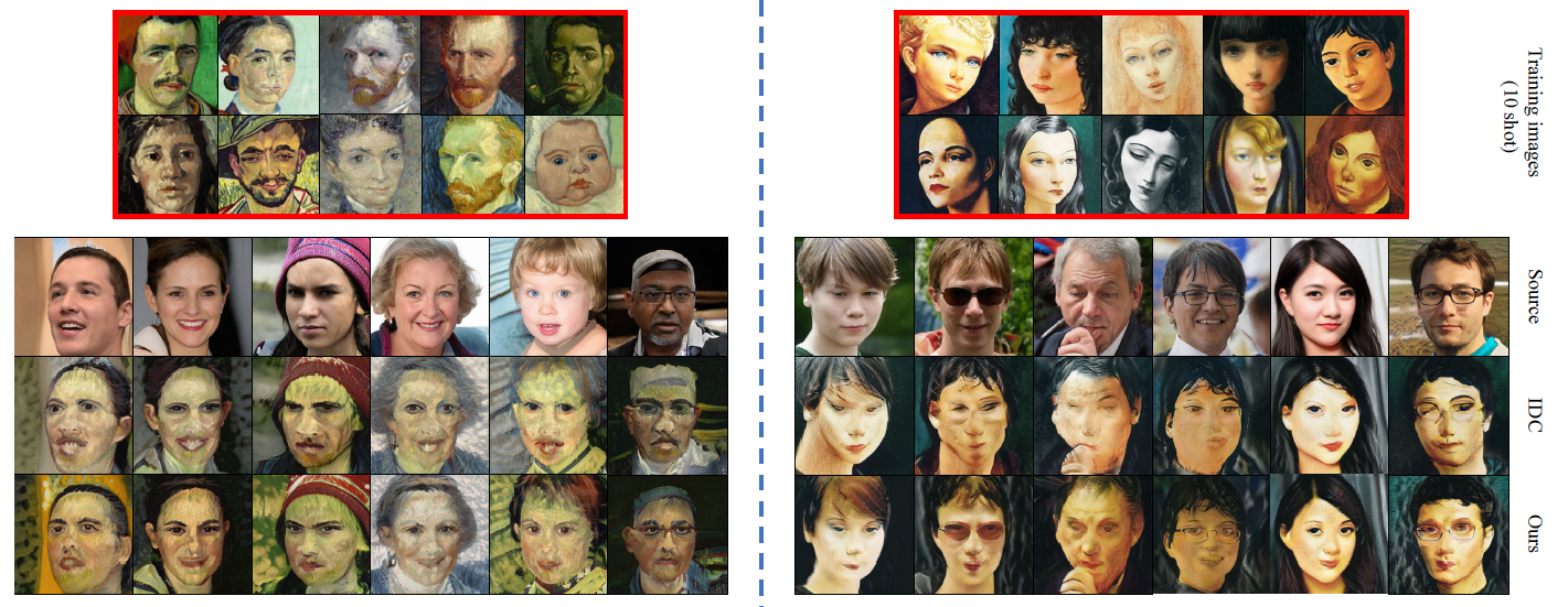

다른 도메인, 다른 수의 학습 이미지를 가지고도 실험한 결과, 본 논문의 방법에서는 distortion이나 texture degradation이 발생하지 않은 것을 확인할 수 있었습니다.

대부분의 실험에서 본 논문의 방법이 IS가 가장 높게 나왔고, 모든 실험에서 SCS가 가장 높게나와 diversity와 quality가 모두 높다는 것을 확인 할 수 있었습니다.

위 그림은 edge map을 IDC에서와 CDC에서 뽑아온 결과인데, 본 논문의 방법이 edge를 더 잘 유지하는 것을 확인 할 수 있었습니다. 따라서, SCS metric도 더 우수하게 나왔습니다.
3.2. Ablation study

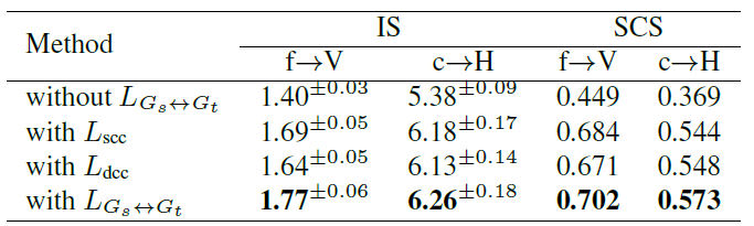
위 사진은 spatial structual consistency loss의 각 요소에 대한 ablation study입니다. \(L_{scc}\)와 \(L_{dcc}\) 모두 image generation을 향상시켰으며 그 둘을 함께 적용시켰을 때 가장 좋은 결과가 나타났습니다.

이번에는 latent space compression의 효과를 알아보기 위한 실험인데, compression을 적용했을 때(with P), target domain과 무관한 속성들 (background, color)가 빠르게 사라지는 것을 확인 할 수가 있었습니다. 이를 통해 latent space compression이 source domain의 attribute를 많이 살려주고 adaption을 빠르게 진행시켜주는 것을 확인 할 수있었습니다.
References
[1] https://arxiv.org/abs/2203.04121
[2] https://openaccess.thecvf.com/content_iccv_2015/papers/Girshick_Fast_R-CNN_ICCV_2015_paper.pdf


댓글